There are easy ways to build adversarial examples that can fool any deep learning model and create security issues. In this post, I’ll show you how an attacker can craft them, and some advice on how to protect against them.
You think it is impossible to fool the vision system of a self-driving Tesla car?
Or that machine learning models used in malware detection software are too good to be evaded by hackers?
Or that face recognition systems in airports are bulletproof?
Like any of us, machine learning enthusiasts, you might fall into the trap of thinking that deep models used out there are perfect.
Well, you are WRONG.
What are adversarial examples?
In the last 10 years, deep learning models have left the academic kindergarten, become big boys, and transformed many industries. This is especially true for computer vision models. When AlexNet hit the charts in 2012, the deep learning era officially started.
Nowadays, computer vision models are as good or better than human vision. You can find them in myriad places, including
- self-driving cars
- face recognition
- medical diagnosis
- surveillance systems
- malware detection
- …
Until recently, researchers trained and tested machine learning models in a laboratory environment, such as machine learning competitions and academic papers. Nowadays, when deployed in real-world scenarios, security vulnerabilities coming from model errors have become a real concern.
Imagine for a moment that the state-of-the-art-super-fancy-deep learning vision system of your self-driving car was not able to recognize this stop sign as a stop sign.
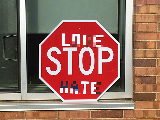
Well, this is exactly what happened. This stop sign image is an adversarial example. Think of it as an optical illusion for the model.
Let us look at another example. Below you have two images of a panda that are indistinguishable to the human’s eye.
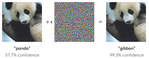
The image on the left is one of the clean images in the ImageNet dataset, used to train the famous GoogLeNet model. The one on the right is a slight modification of the first, created by adding the noise vector in the central image. GoogLeNet predicted the first image to be a panda, as expected. For the second, instead, it predicted (with very high confidence) to be a gibbon. Therefore, it is an adversarial example.
An adversarial example for a computer vision model is an input image with small perturbations, imperceptible to the human eye, that causes a wrong model prediction.
Do not think these are rare edge-case examples found after spending tons of time and computing resources. There are easy ways to generate adversarial examples, and this opens the door to serious vulnerabilities of machine learning systems in production.
Let’s see how you can generate an adversarial example and fool a state-of-the-art image classification model.
How to generate adversarial examples?
Adversarial examples are generated by taking a clean image that the model correctly classifies, and finding a small perturbation that causes the new image to be misclassified by the ML model.
White-box scenario
Let’s suppose you have complete information about the model you want to fool. In this case, you can compute the loss function of the model
J(\Theta, X, y)
where X is the input image, y is the output class, and θ is the vector of the network parameters. This loss function is typically the negative log-likelihood for classification methods.
Your goal is to find a new image X’ that is close to the original X and that produces a big change in the value of the loss function.
Imagine you are inside the space of all possible input images, sitting on top of the original image X. This space has dimensions width x height x channels, so I will excuse you if you cannot visualize it well. To find an adversarial example, you need to walk a little bit in some direction in this space until you find another image X’ with a remarkably different loss. You want to choose the direction that maximizes the change in the loss function J for a fixed small step.
Now, if you refresh a bit your Maths Calculus course, the direction in the X space where the loss function changes the most is precisely the gradient of J with respect to the X.
\nabla_X J(\Theta, X, y) \in \mathbb{R}^{width * height * channels}The gradient of a function with respect to one of its variables is precisely the direction of maximal change. And by the way, this is the reason people train Neural Network using Stochastic Gradient Descent, and not Stochastic Random-Direction Descend :-).
Fast gradient sign method
An easy way to formalize this intuition is as follows:
X' = X + \epsilon *sign(\nabla_X J(\Theta, X, y))
We take only the sign of the gradient and scale it using a small parameter epsilon, to guarantee that the distortion between X and X is small enough to be imperceptible to the human eye. This method is called the fast gradient sign method.
Black-box attack
In most scenarios, it is very likely you will not have complete information about the model. Hence, the previous method is not useful as you cannot compute the gradient.
However, there exists a remarkable property called transferability of adversarial examples that malicious agents can exploit to break a model even if they do not know its internal architecture and parameters.
Researchers have repeatedly observed that adversarial examples transfer quite well between models, meaning that they can be designed for a target model A, but end up being effective against any other model trained on a similar dataset.
Adversarial examples can be generated as follows:
- Query the targeted model with inputs Xi for i = 1 … n and store the outputs yi.
- Use the training data (Xi, yi) to build another model, called the substitute model.
- Use a white-box algorithm like the fast gradient sign to generate adversarial examples for the substitute model. Many of them are going to transfer successfully and become adversarial examples for the target model as well.
A successful application of this strategy against a commercial Machine learning model is presented in this Computer Vision Foundation paper.
Practical example
Let’s get our hands dirty and implement a few attacks using Python and the great library PyTorch. It always comes in handy to know how the attacker thinks.
You can find the complete code in this Github repo.
Our target model is going to be Inception V3, a powerful image classification model developed by Google, which has around 27M parameters and was trained on the popular ImageNet dataset.
# Load pretrained model from the PyTorch hub
# https://pytorch.org/hub/pytorch_vision_inception_v3/
from torchvision.models import inception_v3
model = inception_v3(pretrained=True)
model.eval()

# Count model parameters: 27,161,264
n_params = sum(p.numel() for p in model.parameters())
print(f'{n_params:,} parameters')
We download the list of ImageNet classes the model was trained on, and build an auxiliary dictionary that maps classes ids to labels.
# Download the txt file with the list of ImageNet classes the model was trained with
#     "!" magic to run shell commands from a Jupyter notebook
!wget https://raw.githubusercontent.com/pytorch/hub/master/imagenet_classes.txt

# id2label maps classes ids to their human-readable names: e.g. id2label[1] = 'goldfish'
with open("imagenet_classes.txt", "r") as f:
    categories = [s.strip() for s in f.readlines()]

id2label = {}
for idx, category in enumerate(categories):
    id2label[idx] = category
Let us take the image of an innocent redbone dog as the starting image we will carefully modify to build adversarial examples:
import requests
import io
from PIL import Image

url = 'https://previews.123rf.com/images/meinzahn/meinzahn1211/meinzahn121100339/16350068-cute-tiger-cat-isolated-on-white.jpg'

response = requests.get(url)
img = Image.open(io.BytesIO(response.content))
img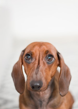
Inception V3 expects images with dimensions 299 x 299 and normalized pixel ranges between -1 and 1.
Let us preprocess our beautiful dog image:
import torch
from torch import Tensor
from torchvision import transforms

def preprocess(img) -> Tensor:
    """
    Inception V3 model from pytorch expects input images with pixel values between -1 and 1
    and dimensions 299 x 299
    """
    mean = [0.485, 0.456, 0.406]
    std = [0.229, 0.224, 0.225]

    preprocess_fn = transforms.Compose([
        transforms.Resize((299,299)),
        transforms.ToTensor(),
        transforms.Normalize(mean, std)
    ])
    image_tensor = preprocess_fn(img)

    # add batch dimension: C x H x W ==> B x C x H x W
    image_tensor = image_tensor.unsqueeze(0)

    return image_tensor

x = preprocess(img)
and check that the model correctly classifies this image.
from easydict import EasyDict
import torch.nn.functional as F

def get_predictions(img: Tensor) -> EasyDict:

    output = model.forward(img)

    class_idx = torch.max(output.data, 1)[1][0].item()

    label = id2label[class_idx]

    output_probs = F.softmax(output, dim=1)
    confidence =  round(torch.max(output_probs.data, 1)[0][0].item(), 4)

    return EasyDict(
        id=class_idx,
        label=label,
        confidence=confidence,
    )

get_predictions(x) # {'id': 168, 'label': 'redbone', 'confidence': 0.8861}
Good. The model works as expected and the redbone dog is classified as a redbone dog :-). Let’s move to the fun part and generate adversarial examples using the Fast Gradient Sign method.
from typing import Tuple
from torch.autograd import Variable

def fast_gradient_sign(x: Tensor, eps: float) -> Tuple[Tensor, Tensor]:
    """"""
    # convert tensor into a variable, because we will need to compute gradients
    # of the loss function with respect to the image pixels
    img_variable = Variable(x, requires_grad=True)

    # forward pass on the original image
    output = model.forward(img_variable)

    # get predicted class
    y_true = torch.max(output.data, 1)[1][0].item()
    target = Variable(torch.LongTensor([y_true]), requires_grad=False)

    # backward pass to compute gradients
    loss_fn = torch.nn.CrossEntropyLoss()
    loss = loss_fn(output, target)

    # this will calculate gradient of each variable (with requires_grad=True)
    # that you can later access with "var.grad.data"
    # PyTorch does the heavy lifting, computing the gradient of the cross-entropy
    # with respect to the input image pixels.
    loss.backward(retain_graph=True)

    # sign of gradient of the loss func (with respect to input X)
    x_grad = torch.sign(img_variable.grad.data)

    # fast gradient sign formula
    x_adversarial = img_variable.data + eps * x_grad

    return x_adversarial, x_grad

# keep epsilon small to generate slight changes to the original image
epsilon = 0.02
x_adv, grad = fast_gradient_sign(x, epsilon)
I have created an auxiliary function to visualize both the original and the adversarial image. You can see the full implementation in this GitHub repository.
visualize(x, x_adv, grad, epsilon)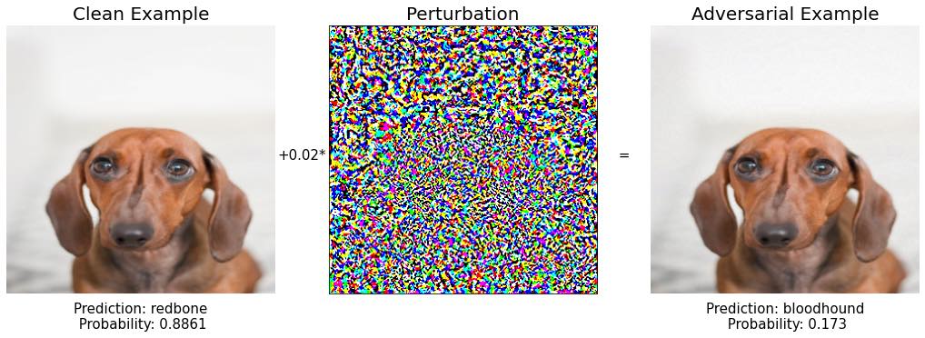
Well. It is interesting how the model prediction changed for the new image, which is almost indistinguishable from the original one. The new prediction is a bloodhound, which is another dog breed with very similar skin color and big ears. As the puppy in question could be a mixed breed, the model mistake seems to be small, so we want to work further to really break this model.
One possibility is to play with different values of epsilon and try to find one that clearly gives a wrong prediction. Let’s try this.
epsilons = [0.02, 0.2, 0.9]
for epsilon in epsilons:
    x_adv, grad = fast_gradient_sign(x, epsilon)
    print('epsilon: ', epsilon)
    visualize(x, x_adv, grad, epsilon)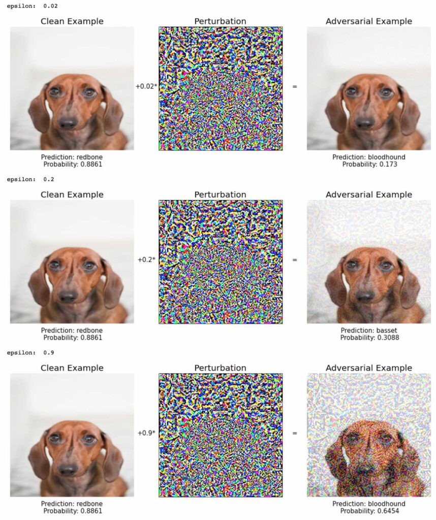
As epsilon increases the change in the image becomes visible. However, the model predictions are still other dog breeds: bloodhound and basset. We need to be smarter than this to break the model.
Remember the intuition behind the Fast gradient sign method, i.e. imagine yourself inside the space of all possible images (with dimension 299 x 299 x 3), right where the original image X is. The gradient of the loss function tells you the direction you need to step to increase its value and make the model less certain about the right prediction. The size of the step is epsilon. You step and you check if you have are now sitting on an adversarial example.
An extension of this would be to take many smaller steps, instead of a single one. After each step, you re-evaluate the gradient and decide the new direction you are going to walk towards. This method is called the Iterative Fast Gradient method. What an original name 🙂
More formally:
X_{n+1} = Clip_{X,\epsilon} [ X_n + \alpha *sign(\nabla_X J(\Theta, X_n, y))]Where X0 = X, and ClipX,ϵ denotes clipping of the input in the range of [X−ϵ, X+ϵ].
A possible implementation in PyTorch is the following:
def iterative_fast_gradient_sign(x_: Tensor, epsilon: float, n_steps: int, alpha: float):
    """"""
    # copy to avoid modifying the original tensor
    x = x_.clone().detach()

    for step in range(n_steps):

        # one step using basic FGSM
        x_adv, grad = fast_gradient_sign(x, alpha)

        # total perturbation
        total_grad = x_adv - x_

        # force total perturbation to be lower than epsilon in
        # absolute value
        total_grad = torch.clamp(total_grad, -epsilon, epsilon)

        # add total perturbation to the original image
        x_adv = x_ + total_grad

        # plot after each iteration
        print('Step ', step + 1)
        visualize(x, x_adv, grad, eps)

        x = x_adv

    return x_adv, total_grad
Now, let us try again to generate a good adversarial example starting from our innocent puppy.
eps = 0.25
n_steps = 9
alpha = 0.025
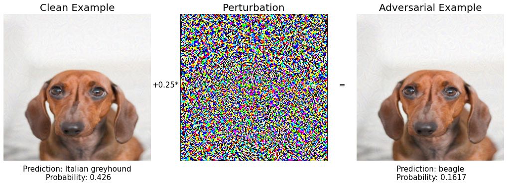
x_adv, grad = iterative_fast_gradient_sign(x, eps, n_steps, alpha)Step 1: bloodhound again..

Step 2: beagle again..
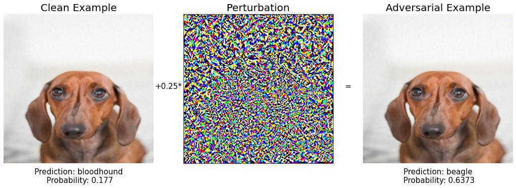
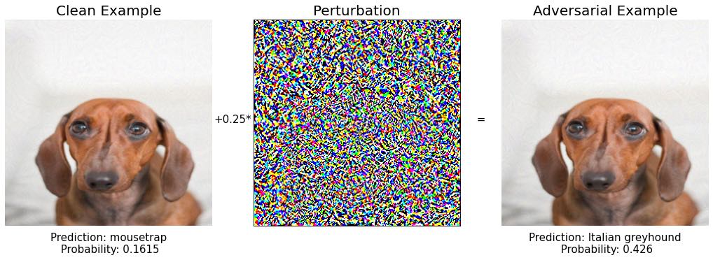
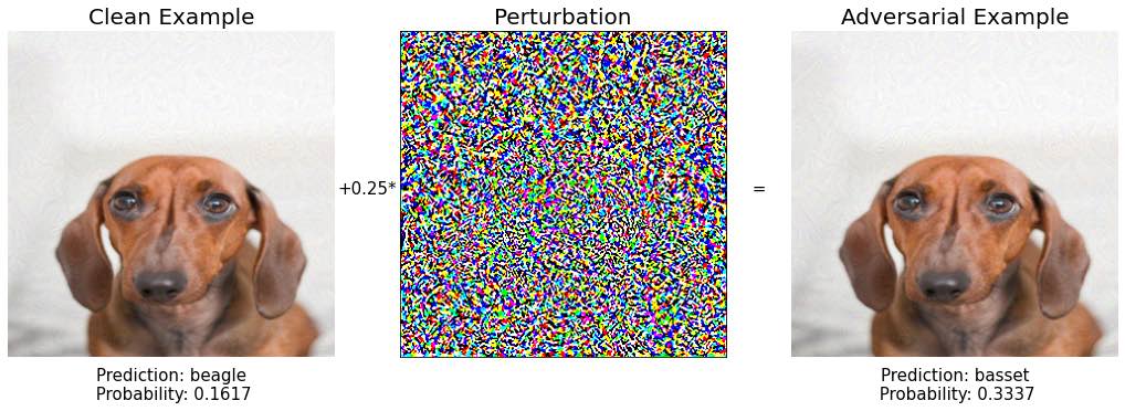
Step 3: mousetrap? Interesting. However, the model confidence on this prediction is only 16%. Let’s go further.

Step 4: One more dog breed, boring…
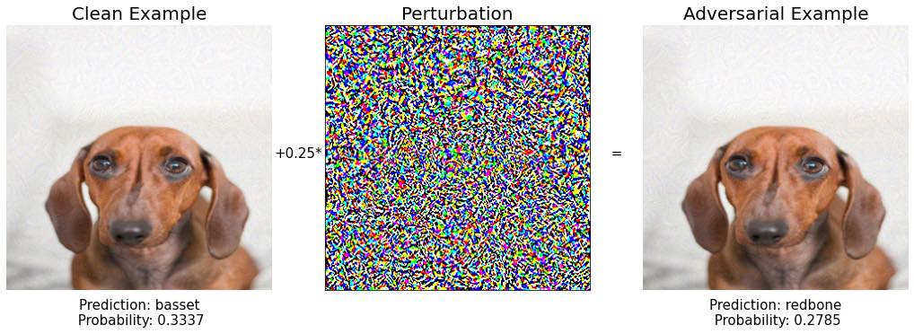
Step 5: beagle again..
Step 6:
Step 7: redbone again.. Keep calm and continue walking in the image space.
Step 8:
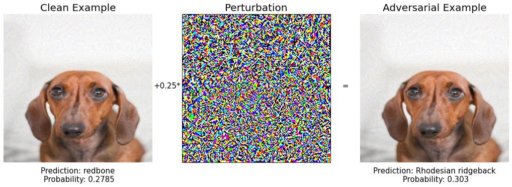
Step 9: BINGO! What an exotic paper towel 🙂 And the model is pretty confident about its prediction, almost 99%.
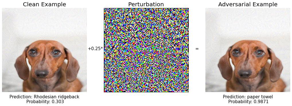
If you compare the initial and the final image we found in step 9
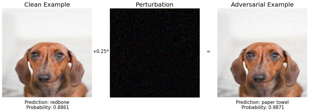
you see they are essentially the same, a puppy, but for the Inception V3 model they are two very different things.
I was very surprised the first time I saw such a thing. How small modifications to an image can cause such model misbehavior. This example is funny, but if you think about the implications for a self-driving car vision you might start to worry a bit.
Deep learning models deployed in critical tasks need to properly handle adversarial examples, but how?
Defenses against adversarial examples
As of June 2021, there is no universal defense strategy you can follow to protect against adversarial examples. In other words, attacking a model with adversarial examples is easier than protecting it.
The best universal strategy, that can protect against any known attack, is to use adversarial examples when training the model.
If the model sees adversarial examples during training, its performance at prediction time will be better for adversarial examples generated in the same way. This technique is called adversarial training.
For example, we could eliminate the adversarial examples we found in the previous section if we added the 10+ examples to the training set and labeled all of them as redbone.
Conclusion
Adversarial examples are a fascinating topic at the intersection of cybersecurity and machine learning. However, it is still an open problem waiting to be solved.
In this post I gave a practical introduction to the topic with code examples. You can check the full code in this Github repo.
If you would like to work further I suggest cleverhans, a Python library for adversarial machine learning developed by the great Ian Goodfellow and Nicolas Papernot, and currently maintained by the University of Toronto.
If you have already been thinking about possible solutions to this problem, get in touch, we can work on it together. You can reach me at plabartbajo@gmail.com.
If you want to read more about machine learning, data science, and freelance, subscribe to the datamachines newsletter or check out my blog