How policy gradients can get you to the moon -

The hands-on RL course – part 7

Policy gradients are a family of powerful reinforcement learning algorithms that can solve complex control tasks. In today’s lesson, we will implement vanilla policy gradients from scratch and land on the Moon 🌗.

If you are new to reinforcement learning, check the introduction to the course to get the fundamentals and jargon in place.

Again, you can find all the code for today’s lesson in this repository 👇🏽

Policy gradients source code — Like it? Give it a **star** on GitHub

Contents

How to get to the Moon with policy gradients? 🚀🌙
The LunarLanderenvironment
Baseline agent
Welcome policy gradients 🤗
Policy gradients agent
Key take-aways
Homework 📚
What’s next?

1. How to get to the moon with policy gradients? 🚀🌙

To land on the Moon we use a spaceship, which is a massive, modular piece of engineering that combines incredible power with gentle precision.

At the beginning of our journey, we use powerful rockets (like the one below) to help the spaceship escape the Earth’s gravitational pull.

Two rockets push our spaceship into space (Photo by Pixabay from Pexels)

Once the rockets are consumed, the spaceship releases them safely into the Earth’s oceans and starts its 385,000 km (239,000 miles) journey to the Moon.

After 3 days our spaceship finally gets close to the Moon and starts orbiting around it. The final act of this masterful play is the landing.

And then, the spaceship releases a device, the lunar lander, that the Moon’s gravitational field pulls downwards towards its surface. What’s more the success of our whole mission depends on a gentle landing of this device.

Lunar Lander device is controlled with Policy Gradients and reinforcement learning — Lunar lander (Wikimedia commons)

In today’s lecture, we will use reinforcement learning to train an agent (aka controller) to land this device on the Moon.

Furthermore, we will use the LunarLander environment from OpenAI as a convenient (and simplified) abstraction of the landing problem.

Finally, this is how the agent you will implement today lands on the Moon.

2. The Lunar Lander environment

Before we get into the modeling part, let’s quickly get familiar with the LunarLander environment.

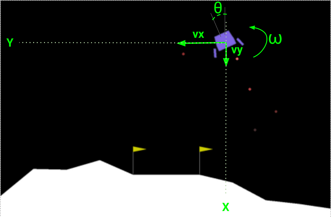
State

The agent gets a state vector with 8 components:

Current position in the 2D world: x and y
Speed along these two axes: vx and vy
Angular position θ with respect to the vertical:
Angular speed ω, that captures the device’s sping around its own axis.
Two binary signals (s1 and s2) to indicate which of the 2 legs of the device (if any) are in contact with the floor.

Policy gradients in the lunar lander environment

Actions

There are 4 possible actions:

0 Do nothing.
1 to fire the left engine.
2 Fire the main engine (central).
3 Fire right engine.

Rewards

In this environment, the reward function is designed to provide enough signals to the agent. This makes training easier.

This is the reward the lander gets at each timestep:

If the lander moves away from the landing pad, it gets negative rewards.
In case of a crash, it receives an additional -100 points.
If it comes to rest, it receives an additional +100 points.
Each leg with ground contact is +10 points.
Firing the main engine is -0.3 points per frame.
Firing the side engine is -0.03 points per frame.
And finally, solved is 200 points.

The pros and cons of reward engineering

Reward engineering is a modeling trick to help RL agents learn, by providing frequent feedback to the agent. Environments with infrequent (aka sparse) rewards are much harder to solve.

However, there are 2 downsides that come with it:

👉🏽 It is hard to design rewards function, as you probably imagined after seeing the LunarLander-v2 reward. There is usually a lot of trial-and-error before one finds the reward function that encourages the agent to learn the right behavior.

👉🏽 Reward shaping is environment-specific, which limits the generalization of the trained agents to slightly different environments. In addition, this limits the transferability of RL agents trained on simulations to real-world environments.

3. Baseline agent

👉🏽 notebooks/01_random_agent_baseline.ipynb

As usual, we get a quick baseline on the problem using a random agent.

Next, we evaluate this agent using 100 episodes to get the total reward and the success rate of the lander:

And then we plot the results

Finally realizing our agent is a complete disaster

Reward average -198.35, std 103.93
Succes rate = 0.00%

*These numbers will not be exactly the same when you run the notebook on your laptop because of the inherent randomness of the agent. In any case, the success rate will be almost surely 0%.

In addition, you can watch a video of this random agent, to convince yourself we are far from solving the problem.

As it turns out, landing on the Moon is not such a piece of cake (what a surprise)

Let’s see how policy gradients can help us land on the Moon.

4. Welcome policy gradients 🤗

The goal of any reinforcement learning problem is to find an optimal policy that maximizes cumulative rewards.

So far in the course, we have used value-based methods, like Q-learning or SARSA. These methods find the optimal policy in an indirect way, by first finding the optimal Q function, and then using this Q function to pick the next-best actions following an epsilon-greedy strategy. This way they come up with the optimal policy.

Policy-based methods, on the other hand, directly find the optimal policy, without necessarily estimating the optimal Q-function.

The 2 basic steps in a policy-based method are the following:

Step 1. Policy parameterization

We use a neural network model to parametrize the optimal policy. This policy is modeled as a stochastic policy, as opposed to a deterministic one. We call it the policy network, and we denote it as

Policy parameterisation for policy gradients — policy depends on parameter θ

Stochastic policies and the exploration/exploitation trade-off

A stochastic policy maps a given observation (input) to a list of probabilities, one for each possible action.

To select which action to take next, the agent samples actions according to their probabilities. As a consequence, stochastic policies naturally handle the exploration vs exploitation trade-off, without hyperparameter tricks like epsilons (as the epsilon-greedy trick used in Q-learning).

In the LunarLander-v2 environment, our stochastic policy will have 8 inputs and 4 outputs. Each of the 4 outputs represents the probability of taking each of the 4 actions.

The architecture of the policy network is a hyperparameter you need to experiment with. The one we will use today has a single hidden layer with 64 units.

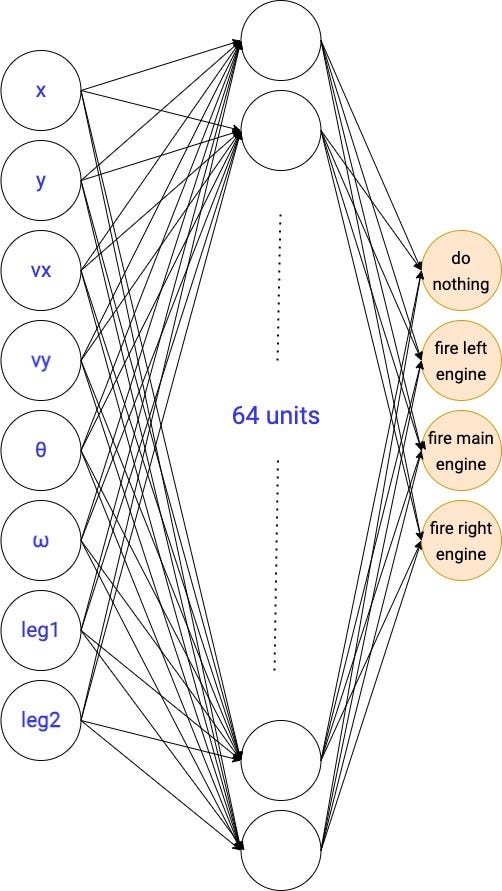
Policy network for our policy gradients agent — Policy network (Image by the author)

Solving our RL problem is equivalent to finding the optimal parameters of this neural network.

But how exactly do we find the optimal parameters for this network?

Step 2. Policy gradients to find the optimal parameters

It is easy to evaluate how good a policy is:

First, we follow this policy for N random episodes and collect the total reward per episode

Second, we average out this N total rewards and get an overall performance measure. This expression is the empirical average of the total reward.

Moreover, the total rewards, and hence J, depend on the policy parameters θ, and our goal is to find the parameters θ that maximize J.

Again, there are different algorithms to solve this maximization problem (e.g. genetic optimization), but as usual in deep learning, gradient-based methods are king 👑.

How do gradient-based methods work?

We start from an initial guess of the policy parameters θ₀ and next, we want to find a better set of parameters, θ₁

The difference between θ₁ and θ₀ is the direction in which we traveled in the parameter space.

The question is, what is the best direction to take to increase J?

And the answer is… the gradient. What is it?

The gradient of a function J with respect to a vector of parameters θ is the direction we need to take from θ to produce a maximal increase of J.

the gradient of J with respect to θ

But, what about the distance we should travel in the gradient direction?

This is another (very popular) hyperparameter: the learning rate α

Equipped with the gradient and a properly tunned learning rate, we do one step of gradient ascent to come up with a better vector of parameters θ₁

Gradient ascent in policy gradients methods — one step of gradient ascent

If we repeat this formula iteratively, we will get better policy parameters and hopefully solve the environment.

And this is how gradient ascent helps us find the optimal policy network parameters.

The remaining question is, how do we compute these gradients?

Estimating the policy gradients

To implement this algorithm, we need an expression for the policy performance gradient that we can numerically compute.

One can mathematically prove, with a little bit of Calculus and Statistics, that the policy parameters can be approximated using a sample of trajectories, collected using the current policy, as follows:

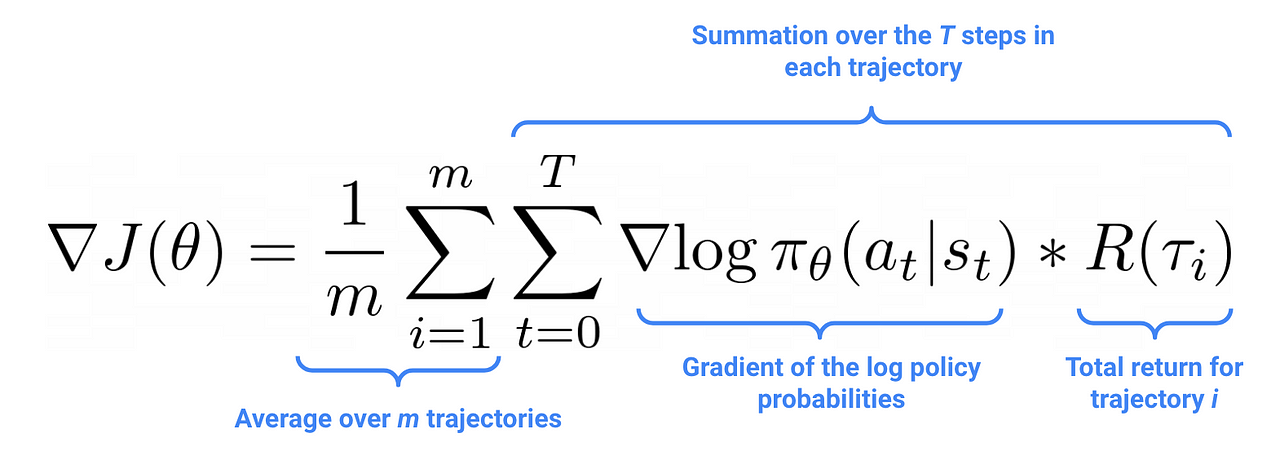
where a trajectory 𝛕 is the sequence of states observed and actions taken until the end of the episode

It is important to stress the fact, that these trajectories have to be collected using the current policy parameters.

On-policy vs off-policy algorithms

Policy gradient methods are on-policy algorithms, which means we can only use experience collected under the current policy to improve the current policy.

On the other hand, with off-policy algorithms, like Q-learning, we can keep a replay memory of trajectories, collected with older versions of the policy, and use them to improve the current policy.

Furthermore, the formula above corresponds to the simplest policy gradients method out there. However, there are variations of this formula, that replace the total return per trajectory R(τᵢ)

with other success metrics.

In particular, there are 2 versions we will see in this course, one today and the other in the next lecture:

The reward-to-go after each action (today)

Reward to go in policy gradients formula

The advantage function (next lecture) which is the difference between the Q function and the V function of the current policy.

Why do we need alternative formulas to estimate the gradient, if we already have one?

All 3 variations of the policy gradient formula have the same expected value, so if you use a very large sample of trajectories, the 3 numbers will be very similar. However, for computational performance we can only afford a small set of trajectories, and hence the variability of these estimates matters.

In particular

👉🏽 the reward-to-go version has a lower variance than the original formula
👉🏽 and the advantage function version has even less variance than the reward-to-go version.

Lower variance results in faster and more stable learning.

Today, we will implement the reward-to-go version, as it is almost as complex as the original vanilla policy gradient formula with cumulative rewards. In the next lecture, we will see how to estimate the advantage function and get even better results.

nd, again, and then, besides, equally important, finally, further, furthermore, nor, too, next, lastly, what’s more, moreover, in addition, first (second, etc.)

Wanna get into the details?
As the purpose of this course is to give you a hands-on approach to the topic, I kept mathematical technicalities to the minimum.
If you want to understand all the steps to derive the policy gradient formula from above, I recommend you read this excellent blog post by Wouter van Heeswijk 📝.

5. Policy gradients agent

👉🏽 notebooks/03_vanilla_policy_gradient_with_rewards_to_go.ipynb

Let’s implement the simplest policy gradient agent out there, where the weights in the policy gradient formula are the episodic rewards.

The hyperparameters are only 3:

learning_rate is the size of the policy gradient updates.
hidden_layers define the policy network architecture.
gradient_weights are the reward-to-go at each time step: i.e. sum of rewards from the current timestep until the end of the episode.

We set up basic logging using Tensorboard and start training our VPGAgent:

The training logic is encapsulated inside the agent.train() function that you can find in src/vgp_agent.py. This function is essentially a loop with n_policy_updates iterations, and in each iteration we:

Collect a sample of batch_size trajectories
Update policy parameters using stochastic gradient ascent.
Log metrics to Tensorboard
Possibly evaluate the current agent, and save it to disk if it is the best agent we found so far.

What is the right batch_size to use?

The number of trajectories per policy update (aka batch_size) is a hyperparameter you need to tune to make sure your training converges to the optimal solution in a reasonable amount of time.

👉🏽 If batch_size is too low you will get very noisy estimates of the gradient, and the training will not converge to an optimal policy.

👉🏽 On the contrary, if batch_size too large, the training loop will slow down unnecessarily, and you will sit and wait 🥱

Plotting training results

While the model is training, we go to the terminal and spin up the Tensorboard server as follows:

$ tensorboard --logdir tensorboard_logs

If you visit the URL printed on the console you will see a chart similar to this, where the horizontal axis is the total number of trajectories collected by the agent so far and on the vertical axis is the total reward per episode.

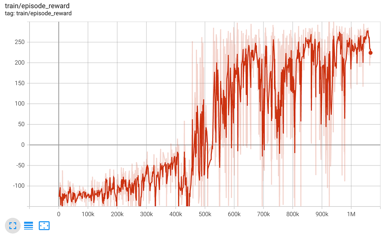
Policy gradients training — Total reward per episode after 1M steps (Image by the author)

We clearly see the agent is learning, and achieves an average total reward around 250 after 1M steps.

As the total reward is not a very intuitive measure, we directly evaluate the agent at the end of training on 100 new episodes, and check the landing success rate:

Reward average 245.86, std 30.18
Succes rate = 99.00%

Wooww! 99% accuracy is pretty good, isn’t it?

Let’s take a quick break, recap and present the homework. Shall we?

Break after policy gradients — Time to take a rest and hydrate (Image by the author)

6. Key takeaways on policy gradients

These are the 3 things I want you to sleep on today:

First, policy gradient (PG) algorithms directly parameterize the optimal policy and tune its parameters using a gradient ascent algorithm.
Second, PG algorithms are more stable (i.e. less sensitive to the hyperparameters), compared to Deep Q-learning, which is good.
And lastly, PG algorithms are less data-efficient, as they cannot reuse old trajectories to update the current policy parameters (i.e. they are on-policy methods). This is something we will need to improve

7. Homework

👉🏽 notebooks/04_homework.ipynb

Can you find a smaller network that solves this environment? I used one hidden layer with 64 units, but I have the feeling this was overkill.
Can you speed up converge by properly tunning the batch_size?

8. What’s next

In the next lesson, we will introduce a new trick to improve the data efficiency of policy gradient methods.

Stay tuned.

Love,

Live.

Learn.

Let’s connect

If you want to learn more about real-world Data Science and Machine Learning subscribe to my newsletter, and connect on Twitter and LinkedIn 👇🏽👇🏽👇🏽